Ion Implant Rs Virtual Metrology: AI-Predicted Sheet Resistance
Key Takeaway
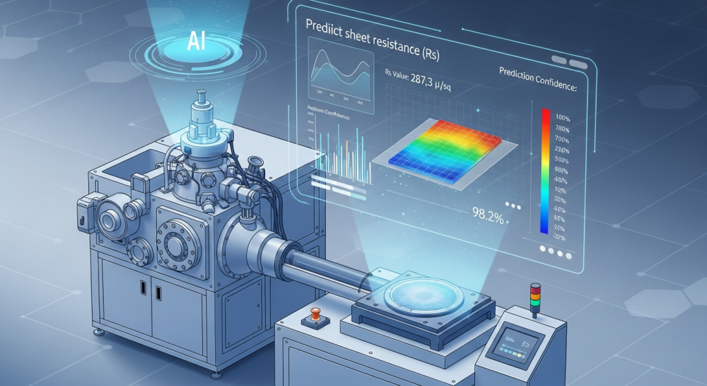
Ion implant sheet resistance can be predicted from beam, dose, energy, scan, vacuum, and thermal context data. Virtual metrology gives fabs earlier visibility into Rs drift and helps prioritize physical measurement when risk or uncertainty is high.
Why sheet resistance matters
Ion implantation controls dopant dose and profile, which directly affect sheet resistance and device electrical behavior. Physical Rs measurement is essential, but metrology sampling and queue time limit how quickly fabs can react. If drift is discovered late, many wafers may already have moved downstream.
Virtual metrology provides an additional layer of monitoring. It predicts Rs from the actual implant process conditions and flags wafers that are likely to be out of target or uncertain enough to require real measurement.
Useful model inputs
- Beam current, dose, dose rate, and beam stability indicators.
- Implant energy, species, tilt, twist, and scan parameters.
- End-station pressure, temperature, and wafer handling context.
- Recipe ID, tool ID, chamber history, PM history, and calibration state.
- Upstream wafer context and post-anneal assumptions when available.
Modeling approach
A practical Rs VM system starts with strong data alignment. Each metrology point must be matched to the correct wafer, lot, recipe, and implant run. The first model can use gradient boosting or a neural network with physical features. The system should output both predicted Rs and confidence, because uncertainty is as important as the point estimate.
When the model is uncertain, the wafer should be sent to physical metrology. When the model is confident and stable, it can increase effective coverage and support faster excursion screening. This fail-closed design is critical for production acceptance.
Operational use
Engineers can use Rs VM to compare chambers, detect beam drift, identify calibration shifts, and decide which lots require immediate measurement. Over time, the VM output can also support run-to-run compensation, but only after shadow-mode validation proves that predictions are stable across recipes, maintenance cycles, and tool states.
读完这篇,下一步可以很具体
获取一份产线 AI 评估,看看 NeuroBox E3200 / SECS/GEM 怎么接到您的设备。
把设备类型、当前数据接口、工艺目标或良率问题发给我们。工程团队会先判断适合 VM、R2R、Smart DOE、EIP 还是能源优化,再给出下一步建议。
- 适合晶圆厂、设备商、工艺/设备/自动化团队
- 可从 SECS/GEM、Modbus、PLC、CSV/历史数据开始
- 不需要先提交机密 recipe 或客户图纸
Deploy real-time AI process control with sub-50ms latency.