SPC & OOC Analysis: Statistical Process Control for Semiconductor Equipment
Key Takeaway
Statistical Process Control (SPC) detects process drift before it causes yield loss using control charts — but 60–70% of OOC alarms in conventional fabs are false positives from improper limit setting. AI-enhanced SPC uses multivariate monitoring and adaptive control limits to cut false alarms while detecting real drifts 30–50% earlier. MST NeuroBox integrates SPC with VM and R2R for closed-loop process stability.
Statistical Process Control is not a new idea. Walter Shewhart invented the control chart at Bell Labs in 1924. Yet more than a century later, the average semiconductor fab still spends 15–25% of its process engineer hours responding to SPC alarms — and the majority of those alarms turn out to be false. This is not a technology problem. It is a problem of applying 1924-era tools to a 2026-era process environment without updating the underlying statistical assumptions.
This article covers the mechanics of SPC as it is actually implemented in leading fabs, explains why standard 3-sigma limit setting produces an unacceptable false-alarm rate in semiconductor contexts, and describes how multivariate monitoring and adaptive control limits restore the original promise of SPC: catch real drift early, ignore noise, and do it automatically.
The Basics: What Shewhart Control Charts Actually Measure
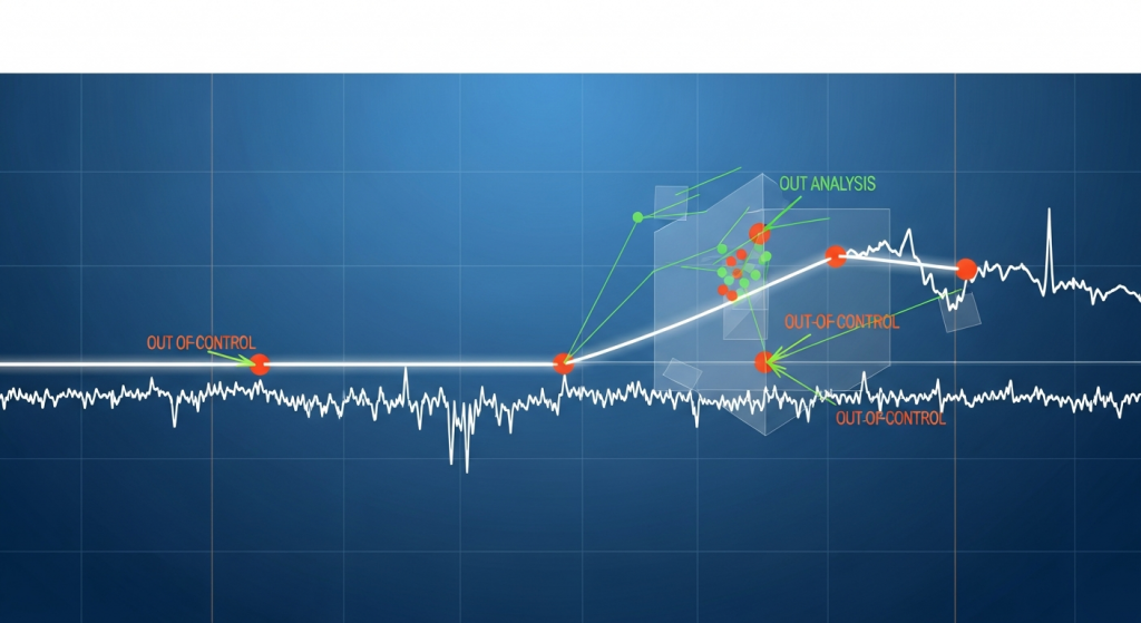
A Shewhart control chart plots a quality characteristic over time alongside a center line (the process mean) and upper and lower control limits (UCL and LCL), typically set at ±3 standard deviations from the mean. Any point outside those limits is flagged as Out-of-Control (OOC), triggering an investigation.
The most common chart types in semiconductor fabs are:
- X-bar chart: Monitors the mean of subgroups. In fab practice, a “subgroup” is usually a batch of wafers run under the same recipe on the same tool. The X-bar chart detects shifts in the process mean.
- R chart (Range chart): Monitors within-subgroup variability by plotting the range (max − min) of each subgroup. Used alongside X-bar to detect increases in spread.
- S chart (Standard deviation chart): Preferred over R for subgroup sizes above 8–10, more statistically efficient at detecting variability shifts.
- EWMA chart (Exponentially Weighted Moving Average): Applies exponentially decreasing weights to past observations, making it more sensitive to small sustained drifts than the Shewhart chart but less sensitive to sudden large jumps. Particularly valuable in CVD and thermal processes where gradual chamber degradation is the dominant failure mode.
- CUSUM chart (Cumulative Sum): Accumulates deviations from target, detecting sustained biases that individual-point rules would miss. Used in diffusion and ion implant where dose drift is slow and continuous.
These charts are built on two core assumptions: (1) observations are independent, and (2) the underlying distribution is approximately normal. Both assumptions are routinely violated in semiconductor manufacturing, and the consequences are severe.
Western Electric Rules and the False-Alarm Inflation Problem
The Western Electric Handbook (1956) extended Shewhart’s single-point rule with additional pattern-detection tests, now universally called Western Electric rules. The most common four applied in fabs are:
- One point beyond ±3σ (original Shewhart rule)
- Two of three consecutive points beyond ±2σ on the same side
- Four of five consecutive points beyond ±1σ on the same side
- Eight consecutive points on the same side of the center line
Each rule, applied individually to a perfectly-in-control process, has a known false-alarm rate. Rule 1 fires by chance once every 370 points (0.27% false-alarm probability per point). But when all four rules are applied simultaneously — which is standard practice — the combined false-alarm rate for a single chart is roughly one alarm every 91.75 points. Apply this to a modern fab running 20–50 SPC charts per critical layer, and the math becomes brutal.
The problem compounds when process data exhibits autocorrelation — consecutive measurements that are not statistically independent. This is almost always the case in semiconductor equipment: chamber conditions at run N influence chamber conditions at run N+1 through residual gas composition, surface chemistry, and thermal state. Autocorrelated data produces tighter apparent control limits than the true process variation warrants, inflating the alarm rate further.
A concrete example: A 300mm etch tool running gate oxide with a measured oxide thickness SPC chart (target: 32Å, σ ≈ 0.4Å) applying all four Western Electric rules will statistically generate a false OOC approximately every 3–4 lots under normal autocorrelated process behavior — before any real process event has occurred. An engineer investigating every alarm would spend roughly 2 hours per shift on SPC dispositions alone.
Why 3-Sigma Limits Are Wrong for Most Semiconductor Applications
Shewhart’s ±3σ limits were derived from a general-purpose industrial context where the cost of investigation was low and sample sizes were large. In semiconductor manufacturing, the asymmetry is the opposite: investigation is expensive (it requires a trained process engineer to pull chamber data, review FDC logs, and potentially hold lots), while the cost of missing a real drift is even higher (yield loss on potentially thousands of wafers).
This creates a fundamental tension that ±3σ limits cannot resolve. Tightening to ±2σ catches more real events but doubles the false-alarm rate. Widening to ±4σ reduces noise but misses early-stage real drifts. The root cause is that a single parameter — sigma width — cannot simultaneously optimize detection sensitivity and false-alarm suppression for all processes and all failure modes.
The correct approach, widely used in advanced fabs, is to set limits based on the process capability index and economic consequences rather than statistical convention. If a process has Cpk = 1.8 (tight distribution well inside spec), the ±3σ control limits will be unnecessarily tight relative to specifications, triggering alarms on variation that poses no yield risk. The control limits should be based on the natural process variation that requires corrective action, not on a fixed sigma multiple.
Multivariate SPC: Hotelling T² for Correlated Parameters
Modern semiconductor processes are not defined by one parameter — they are defined by the interaction among dozens. Etch rate, uniformity, endpoint time, RF reflected power, chamber pressure, and gas flow are all partially correlated. A univariate SPC chart on each parameter individually will:
- Miss drift patterns that only appear in the correlation structure (e.g., etch rate and pressure moving together in a way that is normal for their correlation, but abnormal in absolute terms)
- Generate redundant alarms when one root-cause event shifts multiple correlated parameters simultaneously
Hotelling’s T² statistic addresses both problems. It is the multivariate generalization of the Z-score: it measures the squared Mahalanobis distance of the current observation from the process mean, accounting for the full covariance structure of the parameter set. A single T² control chart then monitors the entire parameter space simultaneously.
The advantages in fab practice are significant:
- Single alarm source: Instead of 15 separate univariate alarms firing in response to one chamber event, a single T² alarm is generated, with a decomposition analysis identifying which parameters drove the excursion.
- Correlation-aware detection: The T² chart detects parameter combinations that are abnormal even when each individual parameter is within its univariate limits. This is the category of “silent” process drift that univariate SPC misses entirely.
- Better false-alarm rate control: With a properly estimated covariance matrix, the T² chart maintains a controlled Type I error rate across all monitored parameters collectively.
The practical challenge with T² is covariance matrix estimation: you need a sufficiently large Phase I dataset (typically 100+ subgroups) under confirmed in-control conditions to get a stable covariance estimate. In new process ramp or after major recipe changes, this requirement can be difficult to meet.
Adaptive Control Limits: The AI Enhancement
Traditional SPC control limits are static — computed once from Phase I data and then frozen. This works acceptably for mature, stable processes, but fails in three common semiconductor scenarios:
- Seasonal / predictable drift: Many processes exhibit gradual, predictable drift tied to PM cycles. Chamber conditions after a PM are systematically different from conditions just before PM. Static limits centered on the overall mean will generate spurious alarms immediately post-PM and may miss real drift in the late-PM period.
- Product mix effects: A tool running multiple product types will have different process signatures for each product. Pooled control limits that ignore product type inflate variation and reduce sensitivity.
- Process evolution during ramp: During technology ramp, the process center and variability legitimately evolve as engineers optimize the recipe. Static limits become obsolete within weeks.
Adaptive control limits solve this by continuously updating the control limit calculation using a sliding window of recent data, weighted to give more influence to recent observations. The key design choices are:
- Window size: Determines the trade-off between responsiveness and stability. Typical values in etch/CVD: 30–60 lots.
- Anomaly-robust estimation: The window must exclude confirmed OOC points from the limit recalculation, otherwise real excursions will progressively widen the limits and mask future drift.
- PM-cycle alignment: Advanced implementations reset the adaptive window at each PM event, building separate control models for early-PM, mid-PM, and late-PM chamber states.
MST NeuroBox’s SPC module implements adaptive limits with PM-cycle awareness, automatically stratifying the control model by chamber age (lots-since-PM) and flagging when the current chamber age has insufficient history for reliable limit estimation.
Field result: A 12-inch power device fab using NeuroBox adaptive SPC on PECVD SiN deposition reduced total SPC alarm volume by 54% within 60 days of deployment, while simultaneously catching two genuine chamber drift events that previous static-limit charts had not flagged until after specification exceedances occurred.
OOC Response Workflow: OCAP and Structured Disposition
An OOC alarm that is not acted upon in a defined, traceable way is operationally worthless. The industry-standard framework for structuring alarm response is OCAP: Out-of-Control Action Plan.
An OCAP is a decision tree that guides the engineer from alarm detection through root-cause identification to corrective action. A well-designed OCAP for a single SPC chart typically contains:
- Triage questions (T = 0–15 min): Is the alarm on a single run or sustained over multiple runs? Is the same parameter alarming on other chambers? Has there been a recent PM, recipe change, or consumable swap?
- Data pull instructions: Specific FDC parameters to review, specific process parameters to compare against baseline.
- Decision nodes: Branch logic for the most common root causes (contamination, chamber wall condition, consumable wear, gas line issue, recipe version mismatch).
- Corrective actions: Specific actions for each identified root cause, with estimated downtime and risk level.
- Lot hold / release criteria: Explicit rules for when to hold affected lots pending further analysis versus when to release to next process step.
The critical integration point is between the SPC system and the MES (Manufacturing Execution System). When an OOC is confirmed after OCAP triage, the MES lot hold must be triggered automatically for all lots processed on the affected chamber since the last confirmed in-control point. Manual lot hold initiation is too slow — in a high-throughput fab, 30–60 minutes of continued processing on an out-of-control tool represents significant yield risk.
| OCAP Stage | Time Target | Key Activity | Responsible |
|---|---|---|---|
| Initial triage | 0–15 min | Confirm alarm, check for obvious causes | Shift engineer |
| Data investigation | 15–60 min | FDC review, chamber comparison, history pull | Process engineer |
| Root cause determination | 1–4 hrs | Identify specific failure mechanism | Senior engineer |
| Corrective action | Variable | Chamber conditioning, PM, recipe adjustment | Process + Equipment |
| Re-qualification | 2–8 hrs | Monitor lots, confirm return to control | Process engineer |
| Lot disposition | Per hold policy | Review held lots, approve release or scrap | Yield / QE team |
SPC on Virtual Metrology Predictions
Traditional SPC can only be applied to physical metrology measurements, which means there is an inherent delay between process execution and process control signal. For a tool processing 24 lots per day with metrology sampling at 25% (6 measured lots per day), each lot waits an average of 2 hours for a control signal. During that time, additional lots continue to run on a potentially drifting process.
Virtual Metrology (VM) eliminates this latency. VM uses a machine learning model trained on process sensor data (FDC traces, chamber signals, endpoint data) to predict the metrology outcome for every run — not just the measured 25%. The SPC chart can then be applied to VM predictions rather than physical measurements, providing 100% run coverage with zero measurement delay.
The implications for OOC detection are substantial:
- 4× more data points per day on a typical 25%-sampled process, dramatically improving the statistical power to detect small shifts.
- Real-time alarm generation: OOC signals are generated within minutes of run completion, not hours later when the wafer completes metrology.
- Lot containment improvement: With real-time OOC detection, the average number of lots processed between a true process event and a lot hold drops from 6–12 lots (physical metrology) to 1–2 lots (VM-based SPC).
The caveat is that VM predictions are model outputs, not direct measurements. SPC on VM predictions should be validated against physical metrology SPC, and the VM model’s prediction uncertainty must be factored into control limit setting. NeuroBox implements dual-layer SPC: VM-based charts for real-time monitoring and physical metrology charts for model drift detection, with automatic reconciliation between the two.
How NeuroBox SPC ties together:
NeuroBox E3200 collects FDC data from equipment → VM model predicts metrology outcome for every run → Adaptive SPC charts monitor VM predictions in real time with PM-cycle-stratified limits → T² multivariate chart monitors the full FDC parameter space simultaneously → OOC alarms trigger OCAP workflow with automated MES lot hold → R2R controller uses the same SPC data stream to adjust recipe setpoints before the next lot runs.
The result is a closed-loop system where SPC is not just a monitoring tool but an active input to process control.
Integration with MES Lot Hold: Closing the Control Loop
The MES integration is where SPC transitions from a reporting tool to a process control tool. The key design principle is: the SPC system must be able to initiate lot holds without human action when the alarm severity and OCAP rules call for it.
This requires three infrastructure components:
- Bidirectional MES interface: The SPC system must receive lot tracking data from MES (to know which lots ran on the alarming tool) and must be able to write lot status changes back to MES (to initiate holds).
- Alarm severity classification: Not all OOC events warrant immediate lot hold. A P1 event (point beyond ±3σ confirmed by OCAP triage) warrants automatic hold. A P2 event (Western Electric pattern rule, first occurrence) may trigger an alert and a 2-hour investigation window before hold escalation.
- Traceable audit log: Every lot hold, every alarm disposition, and every OCAP step must be recorded with timestamp and operator ID. This is required for both internal yield analysis and customer quality documentation.
Fabs that implement automated lot hold based on SPC alarms typically see a 40–60% reduction in the number of out-of-spec lots that escape to downstream process steps, because the containment window shrinks from 2–4 hours (manual process) to 15–30 minutes (automated).
Real Numbers: SPC Performance Benchmarks
To contextualize the improvement potential from AI-enhanced SPC, the following benchmarks come from industry data across multiple 8-inch and 12-inch fabs:
| Metric | Conventional SPC | AI-Enhanced SPC (NeuroBox) |
|---|---|---|
| False alarm rate (% of total alarms) | 60–70% | 15–25% |
| Time to detect real process drift | 4–8 hrs (physical metrology) | 30–90 min (VM-based) |
| Lots affected per OOC event | 8–15 lots average | 2–4 lots average |
| Engineer hours per alarm disposition | 2–4 hrs | 0.5–1.5 hrs (OCAP-guided) |
| OOC alarms reviewed per engineer per day | 8–15 | 2–5 |
| Process Cpk improvement (12-month) | Baseline | +0.15–0.25 Cpk points |
The Cpk improvement deserves emphasis: a 0.2 Cpk improvement on a critical layer (from 1.3 to 1.5) corresponds to a defect rate reduction of roughly 3× on a near-normal distribution, which at 10,000 wafers/month translates to hundreds of additional good wafers per month at a process with meaningful spec exceedance probability.
Implementation Roadmap: Getting SPC Right
For fabs looking to improve their SPC implementation, the following sequence has proven effective in MST deployments:
- Phase 1 — Alarm audit (weeks 1–2): Categorize the last 90 days of OOC alarms as true positive, false positive, or indeterminate. Identify the top 5 charts by alarm volume. This baseline is essential for measuring improvement.
- Phase 2 — Limit recalibration (weeks 3–6): Replace static ±3σ limits with process-capability-based limits on the highest-alarm-volume charts. Implement PM-cycle stratification on etch and CVD tools.
- Phase 3 — OCAP development (weeks 5–10): Build structured OCAP decision trees for the top 10 alarm types. Integrate with MES for automated lot hold on P1 events.
- Phase 4 — VM integration (weeks 8–16): Deploy VM models on high-volume tools and route VM predictions to SPC charts alongside physical metrology data. Validate prediction accuracy and adjust VM model control limits accordingly.
- Phase 5 — Multivariate monitoring (weeks 12–20): Implement T² charts on tools with well-characterized FDC parameter sets. Use T² for early-warning detection and univariate charts for root-cause diagnosis.
The full roadmap takes 4–6 months for a typical fab. MST NeuroBox compresses this timeline significantly because the VM, FDC, SPC, and R2R modules are pre-integrated — the infrastructure connections that typically consume most of the implementation time are already built.
See NeuroBox SPC in Action
MST NeuroBox E3200 integrates adaptive SPC, virtual metrology, and R2R control into a single platform — with MES lot hold automation and OCAP workflow built in.
读完这篇,下一步可以很具体
获取一份产线 AI 评估,看看 NeuroBox E3200 / SECS/GEM 怎么接到您的设备。
把设备类型、当前数据接口、工艺目标或良率问题发给我们。工程团队会先判断适合 VM、R2R、Smart DOE、EIP 还是能源优化,再给出下一步建议。
- 适合晶圆厂、设备商、工艺/设备/自动化团队
- 可从 SECS/GEM、Modbus、PLC、CSV/历史数据开始
- 不需要先提交机密 recipe 或客户图纸
Deploy real-time AI process control with sub-50ms latency.